
Calibrating our solar irradiance sensor for the ParaSol Platform
13 Feb 2026We monitor perovskite solar cells outdoors for months. To tell if a cell is degrading, we need accurate irradiance data. A 5% error in irradiance means a 5% error in calculated efficiency which is enough to confuse real degradation with a bad measurement day.
We use a small (1.18 cm²) commercial monocrystaline silicon cell in short circuit mode assuming that there is a direct proportional constat to translate mA photocurrent from the cell measured by Perovskino to W/m² power irradiation. But it needs calibration as we observed that calibration changes over time.
Three ways to know the irradiance
We work with three complementary data sources:
The silicon cell is our main sensor. We measure its short-circuit current every 3 seconds. Current is proportional to irradiance, but we need the conversion factor (mA → W/m²). It’s cheap, fast, and has a spectral response similar to the cells we’re testing.
The pyranometer measures total irradiance across visible and near-infrared. It’s the meteorological standard equipment usually disposed in horizontal plane. Our pyranometer is on plane as silicon cell and the output signal is offered in mV (0-5000 mV) ideal for the INA219 embeded in the Perovskino.
CAMS data (Copernicus Atmosphere Monitoring Service) provides satellite-estimated irradiance with one-minute resolution. It is free, more or less global coverage and uses sophisticated atmospheric corrections. The limitation: it can’t see small clouds or local shadows in our horizon.
Our strategy is to use CAMS as a long-term reference to calibrate the silicon cell and the pyranometer when available, and track how the calibration evolves.
 Figure 1: Three complementary data sources for irradiance measurement. The silicon cell and the pyranometer provide high-frequency irradiance local data with our horizon, CAMS offers satellite-based reference, serves as ground-truth validation.
The calibration method
The idea is simple. On a clear day, integrate the sensor current, compare it to the energy CAMS predicts for POA 30º, then calculate the conversion factor.
In practice, there are subtleties. Early morning and late afternoon add noise: low solar angles, building shadows, and the silicon’s spectral response deviates from the actual solar spectrum. So we use only midday hours (typically 10:00 - 16:00) for the fitting and require clear-sky conditions with mean absolute error below 3% (30 W/m² MAE). The algorithm finds the factor that minimizes the error difference between measured irradiance (current × factor) and CAMS irradiance.
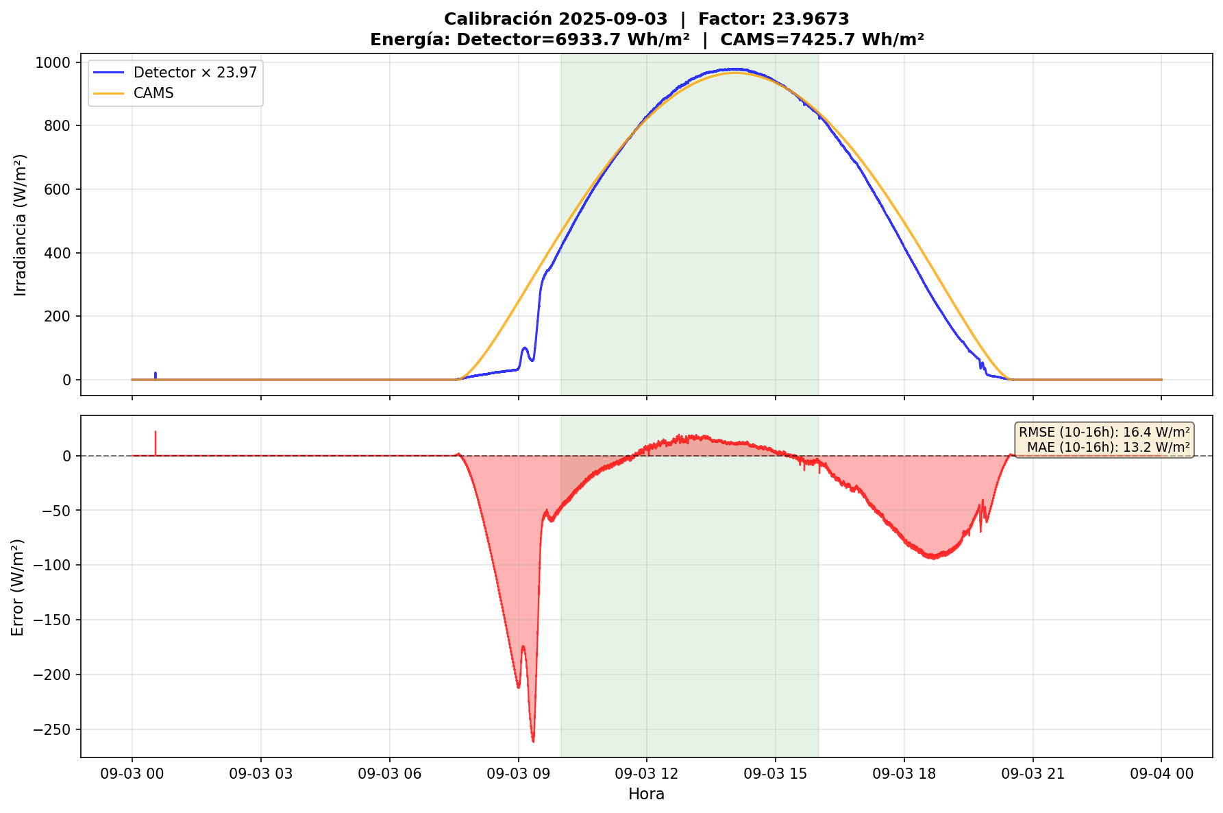 Figure 2: Calibration on a clear day. Top panel shows calibrated sensor signal vs CAMS reference. Bottom panel shows error between both traces. The shaded region marks the midday window used for fitting.
The problem with a single factor
Here’s where it gets interesting. When we calculated the calibration factor daily over 18 months, we didn’t get a constant. The factor drifted.
| Date | Factor |
|---|---|
| June 2024 | 21.0 |
| January 2025 | 19.5 |
| September 2025 | 24.5 |
That’s a 25% variation too large to ignore.
Some variation is noise: cloudy days where CAMS and the sensor see different things, dust accumulation between cleanings, statistical uncertainty. But there’s also a systematic drift that we attribute to encapsulation aging. The epoxi layer protecting our silicon cell yellows and delaminated slightly over time reducing transmission.
Using a single average factor would introduce systematic errors: underestimating irradiance in summer 2024, overestimating it in late 2025. For stability studies spanning months, this affects the efficiency calculations.
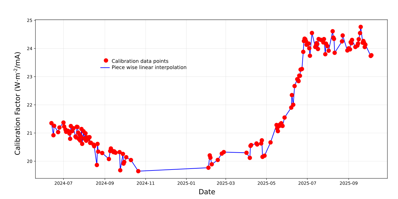 Figure 3: Calibration factor evolution over 18 months. Red points are high-quality days (MAE < 3%) used for the piecewise function. The blue line shows the piecewise linear interpolation.
The solution: a time-varying calibration function
Instead of one factor, we now use a piecewise linear function that interpolates between calibration points. The concept:
- Select high-quality calibration days (clear sky, MAE < 3%)
- For each, record the date and optimal factor
- For any measurement timestamp, interpolate linearly between the two nearest calibration points
- Extrapolate using edge values for dates outside the calibration range
This approach has several advantages:
- Tracks slow drift from encapsulation aging or soiling
- Adapts to seasonal effects in spectral response
- Backward compatible: a single point reduces to a constant factor
- No wild extrapolation: edge values are used conservatively
Why not just use CAMS?
CAMS is great for calibration and long-term validation, but has limitations for real-time monitoring:
- Temporal resolution: 1 minute vs our 3 seconds
- Spatial resolution: ~5 km pixels miss local shadows and small clouds
- Latency: data available hours to days after measurement
- Availability: occasional gaps and outages
The local sensor provides continuous, high-frequency data. CAMS keeps it honest.
The workflow
Our current system works like this:
- Monthly: Run calibration script on recent clear days, add good points to the JSON
- Daily: Export scripts automatically apply piecewise calibration to irradiance data
- On-demand: Analysis scripts use the same calibration for efficiency calculations
 Figure 4: Calibration workflow. CAMS and sensor data feed into periodic calibration runs that update the JSON file. All analysis and export scripts read from this shared calibration, ensuring consistency across the entire data pipeline.
The calibration code is part of our ParaSol outdoor testing platform. If you work on PV characterization and want to compare outdoor stability data across different climates, get in touch.